Looking for a Tutor Near You?

Post Learning Requirement » x
Ask a Question
x

Choose Country Code

x

Direction

x

Ask a Question

x

Hire a Tutor

Cost Notes Lecture All Cost Curves Numerical Examples Theory

Published in: Costing
3,661 Views

For Economics Honors Level Classes

Sourav S / Kolkata

year of teaching experience

Qualification:

Teaches: Abacus Training, Calligraphy, Communicative English, Content Writing, Creative Writing Classes, Handwriting, Indian National Mathematical Olympiad (INMO), Language, Mental Maths, Olympiad Exam Preparation, Personality Development, Regional Mathematical Olympiad (RMO), Speech & Drama, Spell Bee Training, Vedic Maths, Advanced Excel, Basic Computer, Computer for official job, GST Training, MS Office, School level computer, Tally ERP 9, Accent Training, Accounts, Banking & Finance, Book Keeping, BPM Training, Business Analytics, COBIT Certification, Coding & Programming, Customer Service, Data Entry, DSA, E-Commerce, e-Filing, Financial Management, Forex Trading, Freshbooks, Healthcare Management, HR/Personnel, Import & Export, Insurance Training, Investment Training, ITIL Training, Journalism/Writing, Leadership Skills, Marketing Training, MIS Training, PMP Certification, Project Management, Quickbooks, Sales Training, SAP Training, Shipping & Logistics, Six Sigma Training, Soft Skills, Stock & Share Trading, Zoho CRM, ACCA, CA - CPT, CA - Final, CA - IPCC, CA Foundation, CA Intermediate, CFA, CFP, CIMA Certification, CMA Final, CMA Foundation, CMA Intermediate, CMA-CPA-ACCA-CIMA, Corporate Laws, CPFA, CS - Executive, CS - Foundation, CS Professional, Direct Tax Laws, ICWA & ICWAI, Management Subjects, All Subjects, Computer, English, Geography, Hindi, History, Mathematics, Science, Special Education, Accountancy, Algebra, Anthropology, Arts Group, Bio Technology, Biology, Botany, Business Economics, Business Mathematics, Business Organisation, Business Studies, Chemistry, Commerce Subjects, Commercial Arts, Computer Science, Costing, Economics, Education, Enterprenuership, Fashion Study, Food & Nutrition, Home Science, Income Tax, Indirect Tax, Information Practice, IT & Computer Subjects, KVPY Exam, Legal Studies, Logic, Philosophy, Physical Education, Physics, Physiology, Political Science, Psychology, Sociology, Statistics, Zoology, Bengali, EVS, Marathi, NSTSE, NTSE, Actuarial Science, Agriculture, Auditing, B.Arch Tuition, B.Com Tuition, B.Ed Tuition, B.Sc Tuition, B.Tech Tuition, BA Tuition, Bachelor of Tourism Administration, BBA Tuition, BCA Tuition, Behavioral Science, Bio-informatics, Bio-medical, BMS Tuition, BTTM, Business Law, Business Statistics, Civics, Cooperative Accounting, Corporate Accounting, Direct Tax, Electronics, Financial Reporting, General Knowledge, Hotel Management, Human Anatomy, Human Resource, Inorganic Chemistry, IT, M.Com Tuition, M.Ed Tuition, M.Sc Tuition, M.Tech Tuition, MA Tuition, Mass communication, MicroBiology, Organic Chemistry, Pharmacy, Polytechnic, Public Administration, Taxation, ACET, AFCAT, AMAESI, Bank Clerical, Bank PO, CDS/OTA Exam, CSAT, CSEET Exam, CTET, CWE Coaching, Defence Exams, DMRC Entrance, DSSB, EAMCET, EPFO, Food Inspector Exam, Forest Department Exam, GIC, GPSC, GUJCET, IAS Preparation, IBPS, IBPS PO, IES Exam, IISER Exam, Insurance Exams, IPS Exam, ISI Exam, KARTET Exam, KAS Exam, KPSC Exam, LDC Exam, LIC, MHT CET, MPPSC, Municipal Service Commission Exams, NDA, NIRRH, NPTT, NTPC Exam, NTT, PCS Exam, PDO exam, Police Department Exam, PSC Exam, PSU Exam, PTT, PWD & CPWD, Railways Exams, RBI Exam, RRB, RRB JE, RRB NTPC Exam, SBI Exam, School Service Commission, SEBI Exam, SSB Exam, SSC CGL Exams, SSC Exams, SSC JE, Sub-Inspector Exam, TEF Exam, TNPSC, TOPIK Exam, UGC Exams, UPESEAT Exam, UPPSC Exam, UPSC Exam, WBCS, Big Data & Hadoop, Cloud Computing, Data Structures, DBMS & RDBMS, MongoDB, Oracle Training, PL/SQL, Qlikview, R Programming, Tableau, B.Ed, BBA, BCA, MBA, MCA, PG Diploma, AIEEE, AMIE, AMITE, AP EAPCET, AP ECET, Architecture, BCA Entrance, BITSAT, CET, GATE Exam, IIT JAM, IIT JEE Advanced, IIT JEE Mains, JECA Exam, JELET, JEXPO, KEAM, MCA Entrance, NATA Exam, NIMCET, Polytechnic Entrance, TE EAMCET, TS EAMCET, WBJEE, Aeronautical, Aircraft Engineering, Automobile Engineering, Chemical, Civil, Drawing, Electrical, Electronics And Communication, Engineering Graphics, Instrumentation, Mechanical, Mechanics, Production, Simulation Design, Software Engineering, Business English, Corporate Communication, Effective Communication, IELTS, Public Speaking, Spoken English, TOEFL, Musical & Dance Programs, Summer Camps, Training Programs, Workshops & Seminars, Adobe Tools, Corel Draw, DTP, Flash, HTML Training, Multimedia, Page Maker, Photoshop, Special Effects, Video Editing, Kids Gym, Physical Development, Pilates, Play Gym, Yoga, Arts / Crafts, Astrology, Interior Designing, Chinese, Danish, French, German, Administrative Laws, Civil Laws, CLAT, Company Laws, Constitutional Law, Contract Act Laws, Criminal Laws, Jurisprudence, Law Entrance, LLB, LLM, Tax Laws, XLAT Exam, Bachelor of Hospital Administration (BHA), BBA Entrance, BBA Subjects, BBM, BHA, Business Management, Corporate Finance, Finance, Human Resource and Marketing, International Business Marketing, MBA Entrance, MHA, MTTM, AICEE, AIIMS, AIPG Exam, AIPMT, BDS, COMEDK Exam, MBBS Tuition, MCI Exam, MDS Exam, Medical Entrance Exams, NEET, PG Medical, PLAB 1 Exam Preparation, PLAB 2 Exam Preparation, Counting Skills, Drawing / Painting, Nursery Rhymes, Reading Skills, Story Telling, Writing Skills, Phonics, .Net, C, C++, C# (C Sharp), Java And J2EE, Python Programming, Visual Basic, AE Script, Java API, Learning Disabilities, Slow Learners, 3D Printing, Advanced Maths, Lego Programming, Robotics, ACT Exam, FMS, GMAT, GRE, NBDE, NCLEX, NMSQT, OET, PSAT, PTE, SAT, Study in Australia, Study in Canada, Study in China, Study in Dubai, Study in Europe, Study in Germany, Study in Ireland, Study in New Zealand, Study in Norway, Study in Singapore, Study in UK, Study in USA, TOEIC, USMLE, Android Training, Artificial Intelligence (AI), BCA Subjects, Blockchain, Hardware Training, IBM Training, Informatica, IT & Commerce, Networking, SaaS, Software Testing, ACCA Training, ACS, AIEED, AILET, BBE Exam, CAT Exam, CEEB, CEED, CMAT, CUET Exam, DSC Exam, DU JAT Exam, ESI Exam, Fashion Designing, GAT Exam, GOAT, GPAT, Hotel Management Entrance, IBSAT, IFRS, IIFT, IIM Exam, IIMC Entrance Exam, IPMAT, JIPMER, Judicial Services, KMAT, LNAT Exam, LSAT, MAT, MCAT, MICA, MPSC, NEST, NET, NID, NIFT, NIOS, NISM, NMAT, NMIMS Exam, NPAT Exam, PET Exam, SET, SLET Exam, SNAP, TANCET, TET, TIFR, TISS BAT Exam, TISSMAT Exam, TISSNET, UGC Net, XAT, AJAX Training, Digital Marketing, Drupal, Java Script, Joomla Training, Wordpress Training

Contact this Institute
  1. COST BY SOURAV DAS 98367 93076 COST FUNCTION Definition A mathematical formula used to predict the cost associated w!th a ertain action or a certain level of output. use cost functions to forecast the expenses associated with production, in order to determine what pricing strategies to use in order to achieve desired profit margins. The opportunity cost of an asset (or, mor generally, of a choice) is the highest valued opportunity that must be passed up to allow current use Opportunity cost ia also called economic opportunity loss. And is the value of the next best alternative foregone as the result of making a decision Example — I have a TV and VCR. can eithe watch a movie or rent TV and VCR.Out of 2 choices, I am selecting one. In this example; If I w tch movie, then the opportunity cost of watching the movie would be the amount of rent that I would have earned. Explicit costs are expenses for w •ch one must pay with cash or equivalent. Because a cash transaction is involved, they ore relatively easily accounted for in analysis. These costs are never hidden, one has to pay separately. Example- Electricity Bill, wages to workers etc. Implicit costs do not involve a cash transaction, and so we use the opportunity cost concept to measure them. Impllclt costs are related to forgone benefits of any single transaction. These are intangible costs that ayyøpot easily accounted for. Example, the time and effort that an owner puts into the maintenance of the company rather than working on expansion. 1
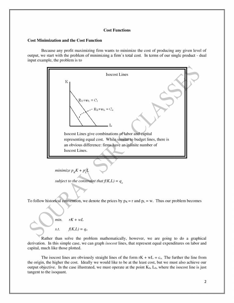
  2. Cost Functions Cost Minimization and the Cost Function Because any profit maximizing firm wants to minimize the cost of producing any given level of output, we start with the problem of minimizing a firm's total cost. In terms of our single product - dual input example, the problem is to Isocost Lines RK+WL Isocost Lines give combinations f labor and capital representing equal cost. While smilarto budget lines, there is an obvious difference: firms hav an infinite number of Isocost Lines. minimize PKK + subject to the constraint thatf(K,L) To follow historical convent on, we denote the prices by r and PL = w. Thus our problem becomes min. s.t. rl
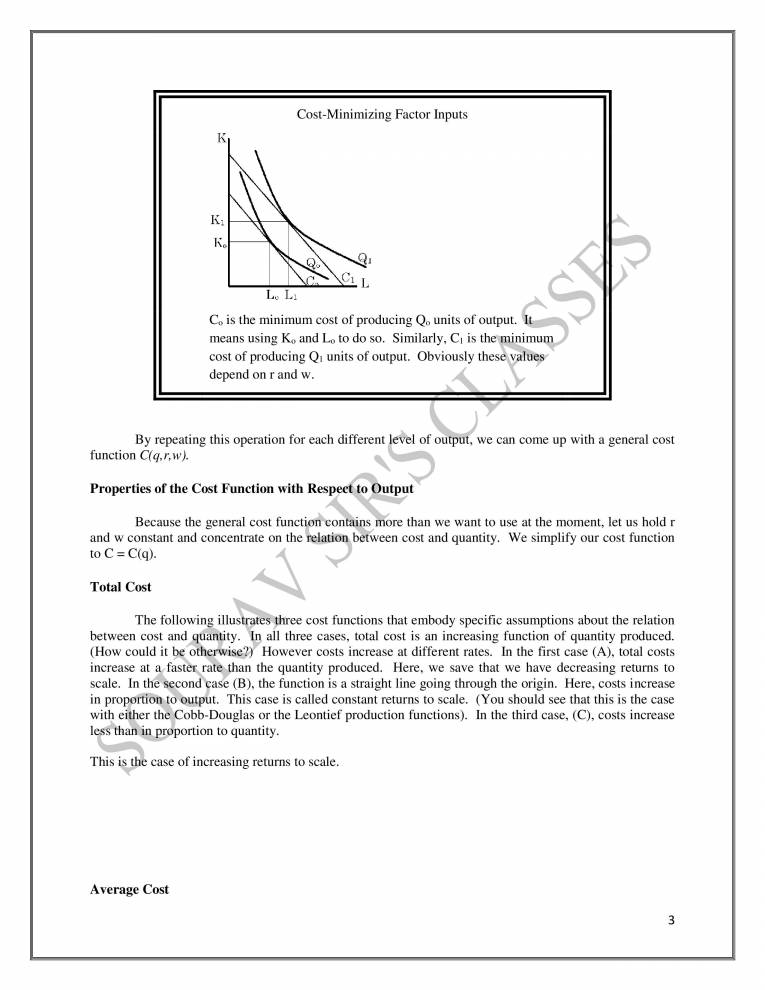
  3. Cost-Minimizing Factor Inputs Co is the minimum cost of producing Qo units of output. t means using Ko and Lo to do so. Similarly, Cl is the inimum cost of producing QI units of output. Obviously thes values depend on r and w. By repeating this operation for each different evel of output, we can come up with a general cost function C(q, r, w). Properties of the Cost Function with Respect to Output Because the general cost function ontains more than we want to use at the moment, let us hold r and w constant and concentrate on the relation between cost and quantity. We simplify our cost function Total Cost The following illustrates three cost functions that embody specific assumptions about the relation between cost and quantity. I all three cases, total cost is an increasing function of quantity produced. (How could it be otherwise?) However costs increase at different rates. In the first case (A), total costs increase at a fasterrate than the quantity produced. Here, we save that we have decreasing returns to scale. In the second gase (B), the function is a straight line going through the origin. Here, costs increase in proportion to output. This case is called constant returns to scale. (You should see that this is the case with either the Cobb-Douglas or the Leontief production functions). In the third case, (C), costs increase les than in roportion to quantity. This •s the case of increasing returns to scale. Average Cost 3
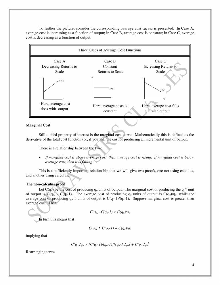
  4. To further the picture, consider the corresponding average cost curves is presented. In Case A, average cost is increasing as a function of output; in Case B, average cost is constant; in Case C, average cost is decreasing as a function of output. Three Cases of Average Cost Functions Case A Decreasing Returns to Scale Here, average cost rises with output Marginal Cost Case B Constant Returns to Scale Here, average costs is constant Case C Increasing Returns o Scale Here, average cost falls with output Still a third property of interest is the marginal cost curve. Mathematically this is defined as the derivative of the total cost function (or, if you Will the cost of producing an incremental unit of output. There is a relationship between the two• • If marginal cost is above average ost, then average cost is rising. If marginal cost is below average cost, then it Is falling. This is a sufficiently important relationship that we will give two proofs, one not using calculus, and another using calculus The non-calculus proof Let C(qj be the cos of producing qo units of output. The marginal cost of producing the qoth unit of output is C(qo) C(qo-l). The average cost of producing qo units of output is while the average ost of producing qo-l units of output is Suppose marginal cost is greater than averag cost. Then C(qo) -C(qo-l) > turn this means that C(qo) > C(qo-l) + implying that Rearranging terms 4
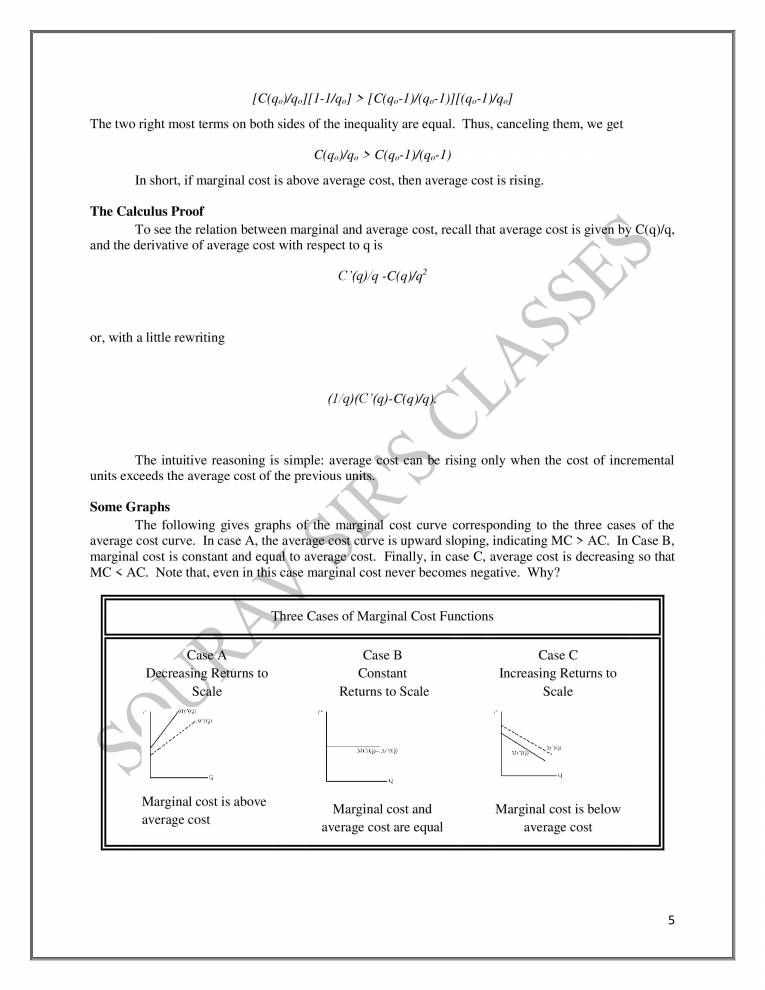
  5. > [C(qo-l )/qo] The two right most terms on both sides of the inequality are equal. Thus, canceling them, we get > C(qo-l In short, if marginal cost is above average cost, then average cost is rising. The Calculus Proof To see the relation between marginal and average cost, recall that average cost is given by C(q)/q, and the derivative of average cost with respect to q is or, with a little rewriting (l q)(C'(q)-C(q)/q The intuitive reasoning is simple: average Oost can be rising only when the cost of incremental units exceeds the average cost of the previous units. Some Graphs The following gives graphs o! th margina cost curve corresponding to the three cases of the average cost curve. In case A, the average cost curve is upward sloping, indicating MC > AC. In Case B, marginal cost is constant and equa to average cost. Finally, in case C, average cost is decreasing so that MC < AC. Note that, even in this c e margmal cost never becomes negative. Why? Three Cases of Marginal Cost Functions Case A Decreasmg RetUrns to Scale Marginal cost is above average cost Case B Constant Returns to Scale Marginal cost and average cost are equal Case C Increasing Returns to Scale Marginal cost is below average cost 5
  6. As you will note, I have drawn marginal cost curves that have constant slope. This need not be the case, as we will see in the case of the U-shaped average cost curve. The U-Shaped Average Cost Curve As a practical matter, most economists believe that the typical competitive firm is characterized by a U-shaped average cost curve, where average cost initially falls as a function of the level of output, reaches a minimum and then begin to rise. At the minimum level of AC, MC = AC. At the minimum AC, the slope of the AC curve is zero, which is sufficient to prove that MC = AC. Finally note that the MC cost curve must cut the AC curve from below. Thus we may draw the average cost curve and the marginal cost curve. The U-Shaped Average Cost Curve Here average cos Irst falls, and then rises. As you can see the marginal cost Curve " uts" the average cost curve at the minimum average cos Note that I have drawn the MC curve so that it is initially falling. This need not be the case, and we have no special Interest in this issue. Fixed and Variab e Cosi It is sometimes useful to divide the firm's costs into fixed and variable components. Fixed costs, FEare the costs the firm would incur if it had no output. That is, FC = C(O). Variable costs are those that vary with output. They may either be defined as the difference between total and fixed costs, VC(q) = C(q) - C(O). It should be obvious that what is defined as "fixed" and "variable" depends on what time period we are talking about. In the long run, there truly are no fixed costs, but in the short run, there may well be. Here is a relation between the average total cost and average variable cost for a U-shaped average cost curve. As you will note 6
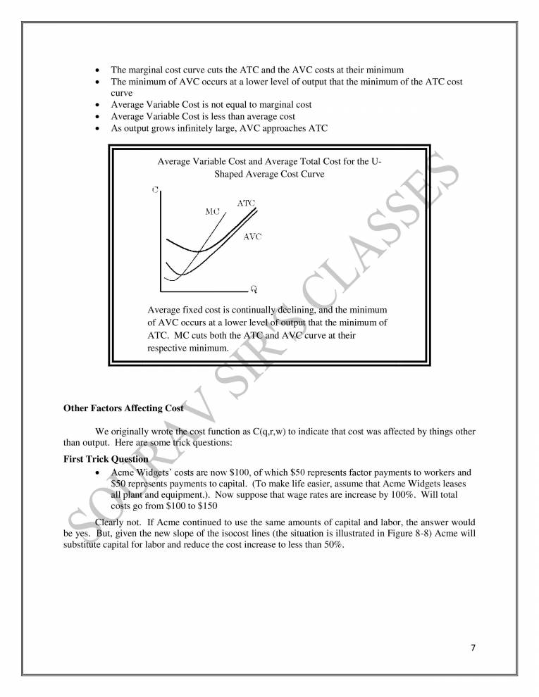
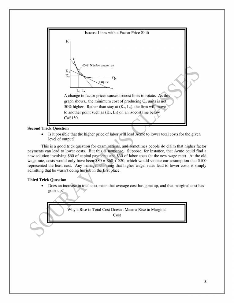
  7. The marginal cost curve cuts the ATC and the AVC costs at their minimum The minimum of AVC occurs at a lower level of output that the minimum of the ATC cost curve Average Variable Cost is not equal to marginal cost Average Variable Cost is less than average cost As output grows infinitely large, AVC approaches ATC Average Variable Cost and Average Total Cost for the U- Shaped Average Cost Curve MC Average fixed cost is continually declining, and the minimum of AVC occurs at a lower level o output that the minimum of ATC. MC cuts both the ATC and A y curve at their respective minimum. Other Factors Affecting Cost We originally wrot the cost function as C(q,r,w) to indicate that cost was affected by things other than output. Here are some Ick questions: First Trick Question cme Widgets' costs are now $100, of which $50 represents factor payments to workers and $50 represents payments to capital. (To make life easier, assume that Acme Widgets leases all plant and equipment.). Now suppose that wage rates are increase by 100%. Will total costs go from $100 to $150 Clearly not. If Acme continued to use the same amounts of capital and labor, the answer would be yes. But, given the new slope of the isocost lines (the situation is illustrated in Figure 8-8) Acme will substitute capital for labor and reduce the cost increase to less than 50%. 7
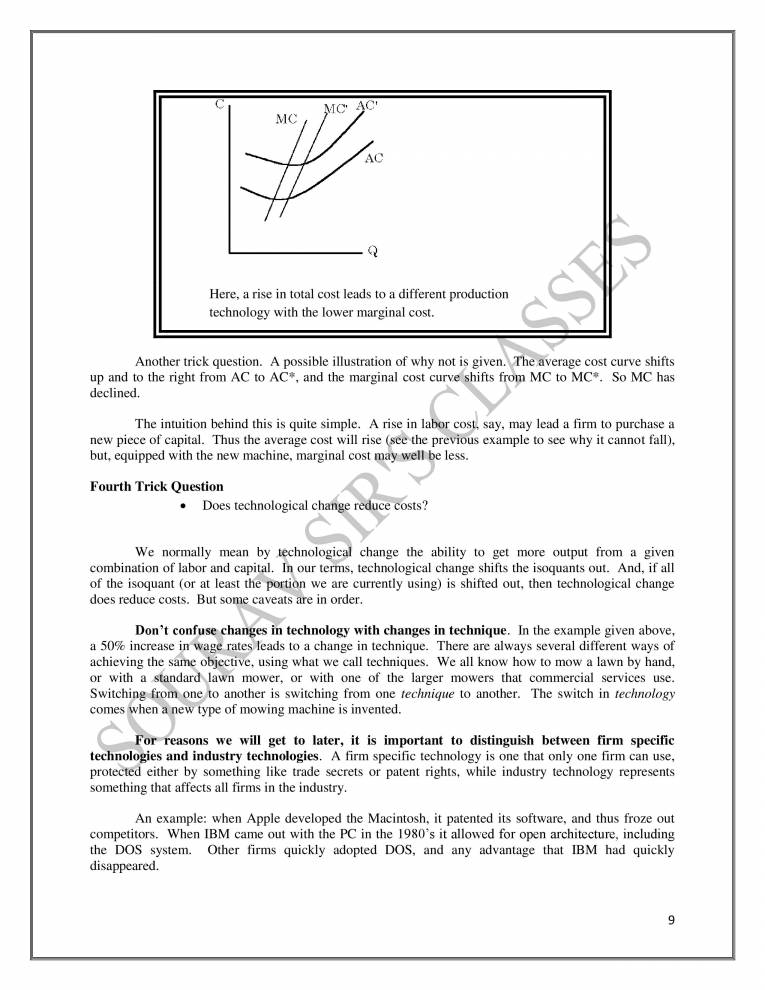
  8. Isocost Lines with a Factor Price Shift wages A change in factor prices causes isocost lines to rotate. As this graph shows, , the minimum cost of producing Qo units is not 50% higher. Rather than stay at (Ko, L), the firm will move to another point such as (Kl, LD on an isocostline below c=$150. Second Trick Question Is it possible that the higher price of labor 111 lead Acme to lower total costs for the given level of output? This is a good trick question for examinations, and sometimes people do claim that higher factor payments can lead to lower costs. But this„is nonsense, Suppose, for instance, that Acme could find a new solution involving $60 of capital payments and $30 of labor costs (at the new wage rate). At the old wage rate, costs would only have beery $80 = $60 + $20, which would violate our assumption that $100 represented the least cost. Any managenclmming that higher wager rates lead to lower costs is simply admitting that he wasn't doing his job in place. Third Trick Question • Does an increase in total cost mean that average cost has gone up, and that marginal cost has gone up? Why a Rise in Total Cost Doesn't Mean a Rise in Marginal Cost 8
  9. C MC Here, a rise in total cost leads to a different production technology with the lower marginal cost. Another trick question. A possible illustration of why not is given. Theaverage cost curve shifts up and to the right from AC to AC*, and the marginal cost curve shifts f om MC to MC*. So MC has declined. The intuition behind this is quite simple. A rise in labor cos say, may lead a firm to purchase a new piece of capital. Thus the average cost will rise (seethe previous example to see why it cannot fall), but, equipped with the new machine, marginal cost ayyell e less. Fourth Trick Question ' Does technological change reduce costs? We normally mean by echnologic change the ability to get more output from a given combination of labor and capital. @our terms, technological change shifts the isoquants out. And, if all of the isoquant (or at least the portion we are currently using) is shifted out, then technological change does reduce costs. But some caveats are in order. Don't confuse changes in technology with changes in technique. In the example given above, a 50% increase Un wage rat. leads to a change in technique. There are always several different ways of achieving the sam objective, using what we call techniques. We all know how to mow a lawn by hand, or with a standar lawn mower, or with one of the larger mowers that commercial services use. Switching from one o another is switching from one technique to another. The switch in technology comes hen a new type of mowing machine is invented. _—ForÄeasons we will get to later, it is important to distinguish between firm specific technologies and industry technologies. A firm specific technology is one that only one firm can use, protected either by something like trade secrets or patent rights, while industry technology represents something that affects all firms in the industry. An example: when Apple developed the Macintosh, it patented its software, and thus froze out competitors. When IBM came out with the PC in the 1980's it allowed for open architecture, including the DOS system. Other firms quickly adopted DOS, and any advantage that IBM had quickly disappeared. 9
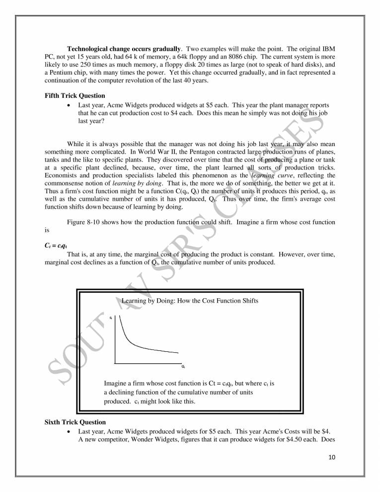
  10. Technological change occurs gradually. Two examples will make the point. The original IBM PC, not yet 15 years old, had 64 k of memory, a 64k floppy and an 8086 chip. The current system is more likely to use 250 times as much memory, a floppy disk 20 times as large (not to speak of hard disks), and a Pentium chip, with many times the power. Yet this change occurred gradually, and in fact represented a continuation of the computer revolution of the last 40 years. Fifth Trick Question • Last year, Acme Widgets produced widgets at $5 each. This year the plant manager reports that he can cut production cost to $4 each. Does this mean he simply was not doing is job last year? While it is always possible that the manager was not doing his job last year, it ma also mean something more complicated. In World War Il, the Pentagon contracted largtproductiovuns of planes, tanks and the like to specific plants. They discovered over time that the cost of producmg a plane or tank at a specific plant declined, because, over time, the plant learned 'all sort of production tricks. Economists and production specialists labeled this phenomenon as the earning curve, reflecting the commonsense notion of learning by doing. That is, the more we do of something, the better we get at it. Thus a firm's cost function might be a function C(qt, Q) the number of units 1 produces this period, q, as well as the cumulative number of units it has produced, Q Thus ove time, the firm's average cost function shifts down because of learning by doing. Figure 8-10 shows how the production function could shift. Imagine a firm whose cost function is Ct = ctqt That is, at any time, the marginal cost of producing the product is constant. However, over time, marginal cost declines as a function of t, t e cumulative number of units produced. Learning by Doing: How the Cost Function Shifts Imagine a firm whose cost function is Ct = ctqt, but where ct is a declining function of the cumulative number of units produced. ct might look like this. Sixth Trick Question • Last year, Acme Widgets produced widgets for $5 each. This year Acme's Costs will be $4. A new competitor, Wonder Widgets, figures that it can produce widgets for $4.50 each. Does 10
  11. this mean that Acme was inefficient? Does it mean that Wonder Widgets stole trade secrets from Acme? Again, Acme may have been inefficient, and Wonder Widgets may have stolen trade secrets from Acme. One can learn a lot by simply observing competitor. If Wonder Widgets simply purchases a widget from Acme, and turns it over to its production specialists for study, there will be a chorus of "So that is what they do!" It is, if you will, just like looking at instructor's old exams. The knowledge will pay off. In fact, there is a general principle: much technological change can confer only a temporary advantage on its developer. We rightly have patent laws to protect new technologies, or else there would be little reason to develop new technology. But the "high tech' firms clearly recogni e that the result of new technology hitting the market is for it to be copied, sometimes)llegally, by! 8ften legally. Thus a high tech firm cannot rest on its laurels, but must continually innovate to keep icost advantage. Applications of Cost Functions to Some Problems of the Firm We can show how some of this material applies by considering two roblems that a firm faces in making production decisions. Allocating output between two different plants The first involves allocating output between two different plants. Suppose a manufacturer has two plants, "A" and "B". The average and marginal coståunctions for the two plants are given in Figure 8-11. As you can see, plant "A" has a higher average cost and a higher marginal cost for each and every level of output than plant "B". While this makes for a nice graph, it is not relevant for management decision making. Marginal and Average Cost for Two Different Plants MCA MCB ACA ACE The example is constructed so that plant "A" has a higher marginal and average cost than plant "B" for every level of output. While this makes for a nice graph, it is irrelevant for decision making. 11
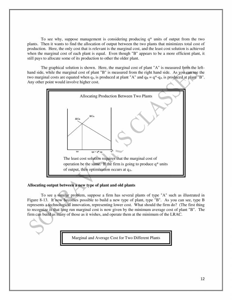
  12. To see why, suppose management is considering producing q* units of output from the two plants. Then it wants to find the allocation of output between the two plants that minimizes total cost of production. Here, the only cost that is relevant is the marginal cost, and the least cost solution is achieved when the marginal cost of each plant is equal. Even though "B" appears to be a more efficient plant, it still pays to allocate some of its production to other the older plant. The graphical solution is shown. Here, the marginal cost of plant "A" is measured from the left- hand side, while the marginal cost of plant "B" is measured from the right hand side. Avou can see the two marginal costs are equated when qA is produced at plant "A" and qB = q*-qA is produced at plan "B" Any other point would involve higher cost. Allocating Production Between Two Plants MCA MCB qB — q*-qA The least cost solution requires that the marginal cost of operation be the same. If the firm is going to produce q* units of output, then optimization occurs at qA. Allocating output between a new type of plant and old plants To see aslmilar pro lem, suppose a firm has several plants of type "A" such as illustrated in Figure 8-13. I now becomes possible to build a new type of plant, type "B". As you can see, type B represents@fechn810gicaf innovation, representing lower cost. What should the firm do? (The first thing to reco;nize is that long run marginal cost is now given by the minimum average cost of plant "B". The firm can build as many of those as it wishes, and operate them at the minimum of the LRAC. Marginal and Average Cost for Two Different Plants 12
  13. ACA MCA MCB ACE L RAC A firm is operating a number of plants of type "A". and it now becomes possible to build new, more efficient plants of type "B". This does not mean the firm should shut down its existing plants, merely change the scale of operation. The existing plants should not begin producing qA units of outpu That does not mean that it should junk its existing plants. It should continue to operate them where the marginal cost equals the new long run marginal cost. Choosing Plant Size Now consider a different problem. firm is considering building one of three different plants, whose average costs are as depicted in Figure 8-i431tS long run average cost curve is then a peculiar scallop-shaped figure, representing the minimum of each of these average cost curves. ong Run Average Cost when Different Sized plants are AC2 possible AC3 ACI A firm can choose between three different plants. Its long run average cost curve is now the scallop-shaped figure, the minimum of the average cost for each of the three plants. 13
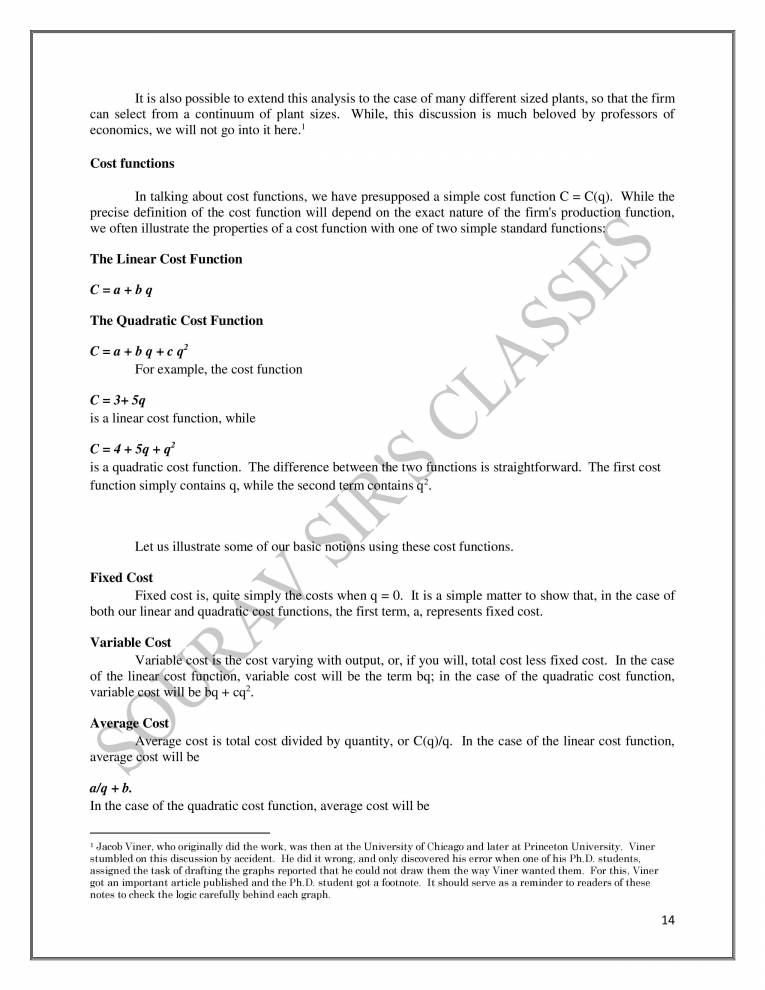
  14. It is also possible to extend this analysis to the case of many different sized plants, so that the firm can select from a continuum of plant sizes. While, this discussion is much beloved by professors of economics, we will not go into it here.l Cost functions In talking about cost functions, we have presupposed a simple cost function C = C(q). While the precise definition of the cost function will depend on the exact nature of the firm's production function, we often illustrate the properties of a cost function with one of two simple standard functions The Linear Cost Function The Quadratic Cost Function C = a + b q +cq2 For example, the cost function is a linear cost function, while is a quadratic cost function. The difference between the two functions is straightforward. The first cost function simply contains q, while the second term contains Let us illustrate some of our basic notions using these cost functions. Fixed Cost Fixed cost is, quite simply the costs when q = 0. It is a simple matter to show that, in the case of both our linear and quadratic cost functions, the first term, a, represents fixed cost. Variable Cost Variable cost is the cost varying with output, or, if you will, total cost less fixed cost. In the case of the linear cost unction, variable cost will be the term bq; in the case of the quadratic cost function, variable ost will be bq + cq . 2 Average Cost _—Äverage cost is total cost divided by quantity, or C(q)/q. In the case of the linear cost function, average cost will be a/q + b. In the case of the quadratic cost function, average cost will be 1 Jacob Viner, who originally did the work, was then at the University of Chicago and later at Princeton University. Viner stumbled on this discussion by accident. He did it wrong, and only discovered his error when one of his Ph.D. students, assigned the task of drafting the graphs reported that he could not draw them the way Viner wanted them. For this, Viner got an important article published and the Ph.D. student got a footnote. It should serve as a reminder to readers of these notes to check the logic carefully behind each graph. 14
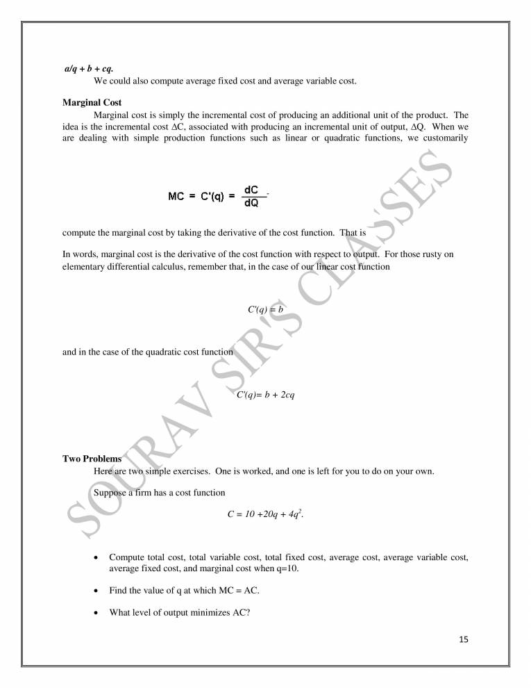
  15. a/q + b + cq. We could also compute average fixed cost and average variable cost. Marginal Cost Marginal cost is simply the incremental cost of producing an additional unit of the product. The idea is the incremental cost AC, associated with producing an incremental unit of output, AQ. When we are dealing with simple production functions such as linear or quadratic functions, we customarily dC MC - C'(q) - compute the marginal cost by taking the derivative of the cost function. That is In words, marginal cost is the derivative of the cost function with respect to utput. For those rusty on elementary differential calculus, remember that, in the case of ouråinear cost unction and in the case of the quadratic cost function Two Problem b + 2cq Here are two simple exercises. One is worked, and one is left for you to do on your own. Suppose a firm has a cost function 2 Compute total cost, total variable cost, total fixed cost, average cost, average variable cost, average fixed cost, and marginal cost when q=10. Find the value of q at which MC = AC. What level of output minimizes AC? 15
  16. Answers At what level of output is marginal cost equal 60? Total cost is 10 + 20 (10) + 4(10)2 = 610. Total variable cost is the last two terms, or 600. Average cost is 10. To compute average cost, average variable cost, and average foxed cost, just divide by 10 to get 61,60, and 1 respectively. Marginal cost is given by 20 + 8q = 100 when q = 10. Average cost is 10/q + 20 + 4q. We want to find the value at which + 20 + = 20 + 8q. Simplifying, we get that and we can solve that equation to get q2 = 2.5, or q = 1.58 • We know that MC = AC at the minimum of the A unction. Thus, from the answer above, we know that the minimum occurs at 1.58. ' Recall that MC = 20 + 8q. That equals 60 when q A Second Problem Suppose the cost function is C = 5+ 10q2. Compute the same answers asked fo above. 1. A person managing dry leaning store for $30,000 per year decides to open a dry cleaning store. The revenues of the store during the first year of operation are $100,000 and the expenses are $35,000 for salaries, $10,000 for supplies, $8,000 for rent, $2,000 for utilities, and $5,000 for interest on a bank loan. Calculate: a. the explicit cost Explicit costs = salaries + supplies + rent + utilities + interest on the bank loan = 35000 + 10000 + 8000 + 2000+ 5000 $60000. b. the implicit costs Implicit costs = entrepreneur forgone salary = $30000. c. the accounting profit 100000 - 60000 = $40000 Accounting profit = TR - explicit costs = d. the economic profit = 100000 - 60000 - 30000 = $10000 Economic profit = TR - explicit costs - implicit costs e. Indicate whether the person should open the dry cleaning store Since the person would earn an economic profit of $10000 per year, he or she should open the dry cleaning store: positive economic profits. 16
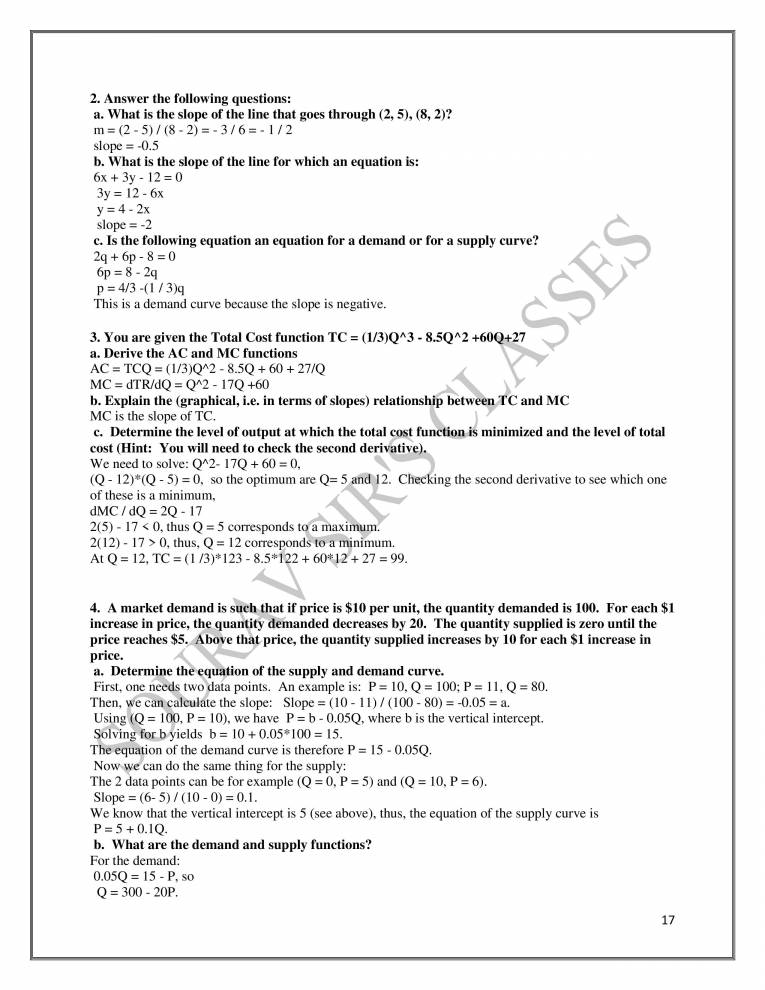
  17. 2. Answer the following questions: a. What is the slope of the line that goes through (2, 5), (8, 2)? 3/6--1/2 slope = -0.5 b. What is the slope of the line for which an equation is: 6x + 3y - 12=0 3y = 12 - 6x y = 4 - 2x slope = -2 c. Is the following equation an equation for a demand or for a supply curve? This is a demand curve because the slope is negative. 3. You are given the Total Cost function TC = (1/3)QA3 - 8.5QA2 +60Q+27 a. Derive the AC and MC functions AC = TCQ = (1/3)QA2 - 8.5Q + 60 + 27/Q MC = dTR/dQ = QA2 - 17Q +60 b. Explain the (graphical, i.e. in terms of slopes) relationship between TC and MC MC is the slope of TC. c. Determine the level of output at which the total cost function is minimized and the level of total cost (Hint: You will need to check the second derivative). We need to solve: QA2- 17Q + 60 = 0, (Q - 12)*(Q - 5) = 0, so the optimum are Q= 5 and 12. Chec •ng the second derivative to see which one of these is a minimum, dMC / dQ = 2Q - 17 2(5) - 17 < 0, thus Q = 5 corresponds to a maximu 2(12) - 17 > 0, thus, Q = 12 corresponds to a minlmum. AtQ= 12, TC = (1 - 8.5*1 2+ 27 = 99. 4. A market demand is such that if price is $10 per unit, the quantity demanded is 100. For each $1 increase in price, the quantity demanded decreases by 20. The quantity supplied is zero until the price reaches $50Åbove that price, the quantity supplied increases by 10 for each $1 increase in price. a. Determine the equation of the supply and demand curve. First, one needs two data points. An example is: P = 10, Q = 100; P = Il, Q = 80. Then, ye can calculate the slope: Slope = (10 - Il) / (100 - 80) = -0.05 = a. Using (Q = 100, P = 10), we have P = b - 0.05Q, where b is the vertical intercept. Solvmg for& ields 10 + = 15. The equation of the demand curve is therefore P = 15 - 0.05Q. Noww can do the same thing for the supply: The 2 data points can be for example (Q = 0, P = 5) and (Q = 10, P = 6). Slope = (6-5) / (10 - 0) = 0.1. We know that the vertical intercept is 5 (see above), thus, the equation of the supply curve is P = 5 +0.1Q. b. What are the demand and supply functions? For the demand: 0.05Q = 15 -P, so Q = 300 - 20P. 17
  18. Similarly for the supply function, inverting the equation of the supply curve yields: Q = -50 + IOP. c. What is the equilibrium price and quantity? Setting demand = supply yields: -50 + IOP = 300 - 20P, 350 = 30P, P = 350/ 30 = $11.67 Plugging in the demand or supply function to get quantities yields Q : = Q = -50+ 10(11.67) = 5. Using the demand function Q = 300 - IOP (1) 66.67. a. Determine the equation of the total revenue (TR), average revenue (AR) and marginal revenue TR = PQ. In order to calculate it, one needs to invert the demand function so that we can find t e demand curve equation: IOP = 300 - Q, P = 30 - o.1Q. Now, if we multiply both side of the demand curve equation by Q, we will have an expression for total revenue: TR = PQ = (30 - = 30Q - o.1Q2 Average revenue is defined as TR / Q: AR = (30Q - 0.1Q2 ) / Q - 0.1 Marginal revenue is defined as the first derivative of total revenue: MR = dTR/ dQ = 30 - 0.2Q b.c. see class notes/ not included d. Determine mathematically at what quantity is total revenue maximized. Check that you have maximized not minimized total revenue. In order to maximize total revenue, one needs to set the first derivative of the total revenue function (the marginal revenue function) equal to 0: 30 - 0.2Q = 0, 30 = 0.2Q, Q = 30 / 0.2 = 150. At quantities of 150, total revenue is optimized. In order to know whether we have a maximum or a minimum,pne needs to check the second derivative: d2TR/ dQ2 = dMR/ dQ = -0.2. Since -0.2 < 0, we conclude that we have maximized not minimized total revenue at Q = 150. SUNK COST Sunk costs are retrospective costs that cannot be recovered, and are therefore irrelevant to future investment decisions in the project which incurs them. CHECKPOINTS o Only prospective costs should impact an investment decision. Therefore, sunk costs are not to be considered when deciding whether to undertake a project. A sunk cost is distinct from an economic loss. A loss may be caused by a sunk cost, however. Sunk costs are irrecoverable. 18
  19. Sunk Costs Examples Let's say a company spent $5 million building an airplane. Before the plane is complete, the managers learn that it is obsolete and no airline will buy it. The market has evolved and now the airlines want a different type of plane. The company can finish the obsolete plane for another $1 million, or it can start over and build the new type of plane for $3 million. What should the managers decide? Should they spend that last $1 Plillion to finish up the plane that's almost done, or should they spend the $3 million to build the new plane. At first glance, you may think the company should just finish the old plane. It's only anothe illi bucks and they already spent $5 million. But in reality, the five million is irrelevant: It is a sunk Cost. The only relevant cost is the $3 million dollars. The managers should consider whether or notto spend $3 million on the new plane, and nothing regarding the old plane should affect the decisio DIFFERENCE BETWEEN SUNK COST AND ECONOMIC LOSS The sunk cost is distinct from economic loss. For example, when a car is purchased, it can subsequently be resold; however, it will probably not be resold fort e Original purchase price. The economic loss is the difference between these values (including transaction co ts). The sum originally paid should not affect ny rational future decision-making about the car, regardless of the resale value. If the owner can derive more alue from selling the car than not selling it, then it should be sold, regardless of the price pai In this sense, the sunk cost is not a precise quantity, but an economic term for a sum paid in the past, which is no longer relevant to decisions about the future. The sunk cost may be used to refer to the original cost or the expecte economic loss. It may also be used as shorthand for an error in analysis due to the sunk cost fallacy irrational decision-making or, most simply, as irrelevant data. Sunk Costs Fallacy The sun cost fallacy is when someone considers a sunk cost in a decision and subsequently makes a poor decision, An example of the sunk cost fallacy is paying for a movie ticket, finding out the movie is terrible, and staying to watch anyway just to get your money's worth. When you find out the movie is terrible, you should make a decision whether to sit through the bad movie or to do something more meaningful with your time — the price you paid for the ticket should not affect your decision. The ticket price is a sunk cost. Another example of the sunk cost fallacy is paying for an all-you-can-eat buffet, eating until you're full and then going back for more just to get your money's worth. When you are full, you should decide 19
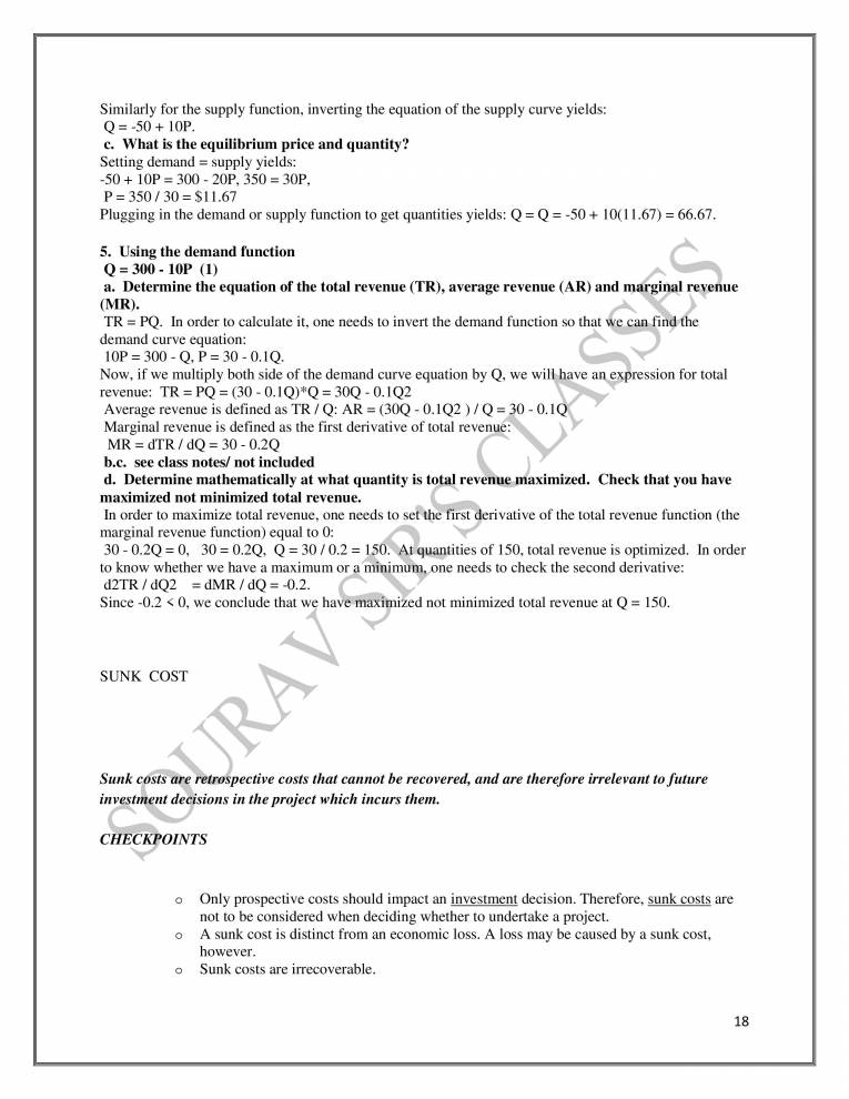
  20. whether you want to eat more or to stop eating the fact that you paid for unlimited food should not affect your decision. The price of the buffet is a sunk cost. COST CURVES Curves can be drawn to represent costs. The marginal cost (MC) and the average cost (AC) are shown in the following diagram (23-3). OX and OY are two axes, along OX is shown the quantity produced and along OY the cost. It will be seen that as output is increased, both average cost (AC) and marginal cost (MC) fall, but MC is below AC, i.e., marginal cost is less than the average cost. The fall is due to the economies of scale. But beyond a point (M), i.e., when output is expanded too much, both AC and MC start rising and now MC is above AC, i.e., the marginal cost is greater than the average cost. That is why MC cuts AC from below at its lowest point. There are two types of other cost curves. They are the Average Variable Cost Curve and the Average Fixed Cost Curve. The average variable cost is obtained by dividing the total variable cost by the number of units produced. Average fixed cost is obtained by dividing the total fixed cost by the total units of output. The total fixed cost being fixed for all units of output, AFC is a falling curve in the shape of a rectangular hyperbola. 20
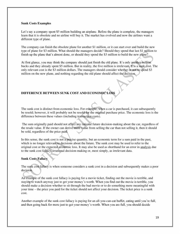
  21. MC OVANTtry Average Cost and Marginal Cost Fig. 23.3 The average variable and average fixed cost curves can be represented as below (Fig. 23-4). OX and OY are the two axes. The output is represented along OX and cost along OY; AFC curve represents average fixed cost. AVC curve represents average variable cost, ATC curve represents average total cost (i.e., total of AFC and AVC and is called AC, i.e., average cost). MC curve represents marginal cost. It is clear that as output is increased, the cost per unit decreases due to various internal economies. That is why AFC, AVC and hence ATC all start falling. But if the output is expanded beyond proper limit, diseconomies will result, and all these costs will go up, which is shown by the rising portions of these curves. This is the third stage of the Law of Variable Proportions. MC ATC AVC ournr (boo YDS) Average. Variable and Fixed Costs Fig. 23.4 It will be seen that AFC continues to fall, it never rises, and rather it helps AVC to fall too for some time, but after some time AVC starts rising quickly and raises ATC too. MC and AVC fall and rise at the same time. But it is to be carefully noticed that when MC and AVC are falling, MC is below AVC, but when they rise, MC is above AVC. When AVC is constant, MC is equal to it. In other words, MC cuts AVC and ATC at their lowest points. 21
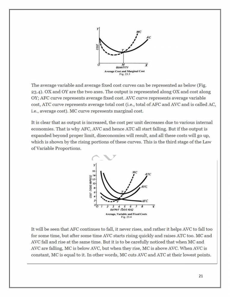
  22. EXPANSION PATH The change in the optimal input bundle when output changes depends on the nature of the production function. The path of all optimal input bundles as output increases is called the output expansion path. The blue line in the following figure is an example of an output expansion path. isoquants isocost lines output expansion path 1 In this example, as output increasei initially mor of both inputs are used. Then, between the second and third isocost lines the amount of input 2 used s arts to decline. If the optimal amount of an input increases with output then the input is called normal, while if the amount used decreases then the input is called inferior. Example: a production function with fixed proportions Consider the production function F (Zl, Q) = min{zl, Q}. Given the shape of its isoquants, the output expansion path of this production function is a ray from the origin, as in the following figure. For any input prices the firm uses y units of each input to produce y units of output (see its conditional input demands), so that its output expansion path is the line z2 = Zl. 22
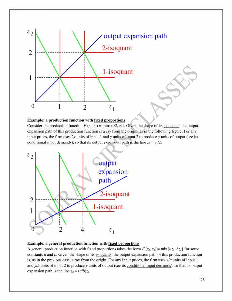
  23. 2 1 1 2 output expansion path 2-isoquant I -isoquant 1 Example: a production function with fixed proportions Consider the production function F (Zl, Q) = min{z1/2, Q}. Given the hape of its isoquants, the output expansion path of this production function is a ray from the orig@as m the following figure. For any input prices, the firm uses 2y units of input 1 and y units of input 2 to produce y units of output (see its conditional input demands), so that its output expansion path 's the line = Zl/2. output expansion path 2 1 2 4 2-isoquant I -isoquant 1 Example: a general production function with fixed proportions A general production function with fixed proportions takes the form F (Zl, Q) = min{azl, be} for some constants a and b. Given the shape of its isoquants, the output expansion path of this production function is, as in the previous case, a ray from the origin. For any input prices, the firm uses y/a units of input 1 and y/b units of input 2 to produce y units of output (see its conditional input demands), so that its output expansion path is the line = (a/b)zl. 23
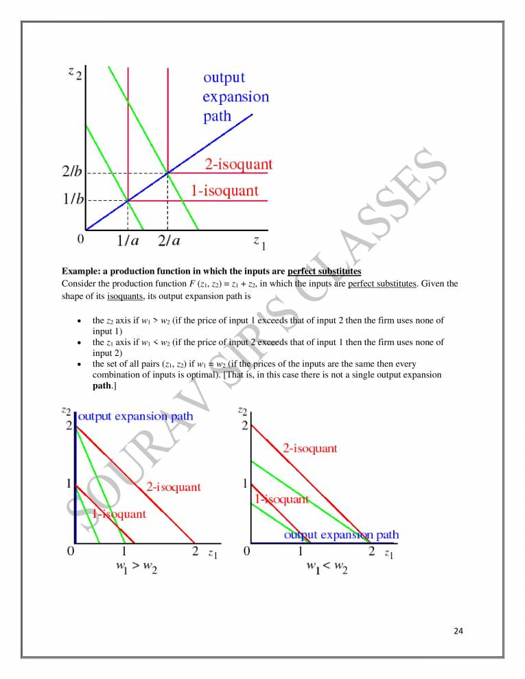
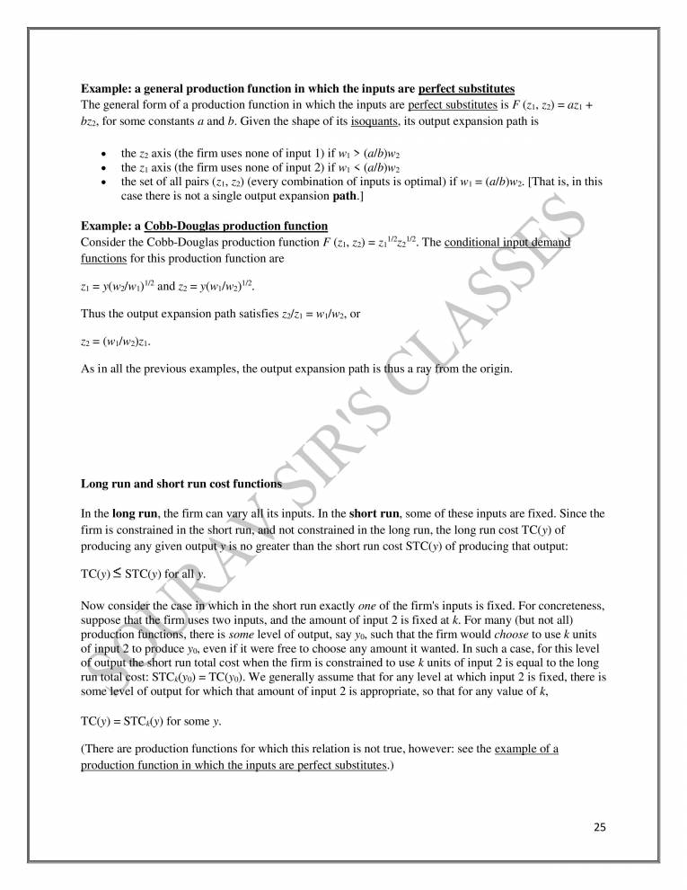
  24. 21b 11b o l/a 2/a output expansion path 2-iso uant I-isoquant 1 Example: a production function in which the inputs are perfect substitutes Consider the production function F (Zl, Q) = + Q, in which the inputs are perfect substitutes. Given the shape of its isoquants, its output expansion path is the axis if WI > (if the price of input 1 exceeds that of input 2 then the firm uses none of input 1) the axis if WI < (if the price o!input 2 exceeds that of input I then the firm uses none of input 2) the set of all pairs (Zl, Q) if WI vv'2 (if the prices of the inputs are the same then every combination of inputs is optimal). [That IS, in this case there is not a single output expansion 2 1 path.] output expansion path 2-i sciluant quant 2 1 1 w 2 2-isoquant o ut expan 1 path 24
  25. Example: a general production function in which the inputs are perfect substitutes The general form of a production function in which the inputs are perfect substitutes is F (Zl, Q) be, for some constants a and b. Given the shape of its isoquants, its output expansion path is = LIZ 1 + the axis (the firm uses none of input l) if WI > (a/b)vv2 the axis (the firm uses none of input 2) if WI < (a/b)W'2 the set of all pairs (Zl, Q) (every combination of inputs is optimal) if WI = (a/b)w2. [That is, in this case there is not a single output expansion path.] Example: a Cobb-Douglas production function Consider the Cobb-Douglas production function F (Zl, a) functions for this production function are = and = Thus the output expansion path satisfies z2/z1 = WI/W2, or Z2 = (WI/W2)Zl. 1/2 1/2 = Zl z2 . The conditional input demahd As in all the previous examples, the output expansion path is t us ara from the origin. Long run and short run cost functions— In the long run, the firm can vary allits inputs. In the short run, some of these inputs are fixed. Since the firm is constrained in the short run, and not constrained in the long run, the long run cost TC(y) of producing any given outpu y is no greater than the short run cost STC(y) of producing that output: TC(y) STC(y) fo ally. Now consider the case in which in the short run exactly one of the firm's inputs is fixed. For concreteness, suppose that the firm ses two inputs, and the amount of input 2 is fixed at k. For many (but not all) produc ion functions, there is some level of output, say yo, such that the firm would choose to use k units of in ut 2 to produce yo, even if it were free to choose any amount it wanted. In such a case, for this level o output the sßort run total cost when the firm is constrained to use k units of input 2 is equal to the long run total fost: STCk(yo) = TC(yo). We generally assume that for any level at which input 2 is fixed, there is som&level of output for which that amount of input 2 is appropriate, so that for any value of k, TC(y) = STCk(y) for some y. (There are production functions for which this relation is not true, however: see the example of a production function in which the inputs are perfect substitutes.) 25
  26. For a total cost function with the typical shape, the following figure shows the relations between STC and TC. STCk TC Examples of long run and short run cost functions Long run and short run average cost functions Given the relation between the short and long run tota costs, the short and long run average and marginal cost functions have the forms shown in the following igure SAC LAC LMC SMC Note: The SMC goes through the minimum of the SAC and the LMC goes through the minimum of the LAC. 26
  27. When SAC = LAC we must have SMC = LMC (since slopes of total cost functions are the same there). In the case that the production function has CRTS, the LAC is horizontal, as in the following figure. LAC = LMC SMC Derivation of Long-Run Marginal Cost Curve The Derivation of Long-Run Marginal Cost Curve! SAC Since marginal cost curve is important 0th from the viewpoint of the short run and the long run, it will be useful to know how the long-ru marginalcost curve is derived. The long-run marginal cost curve can be directly derived from the long-run total cost curve, since the long-run marginal cost at a level of output is given by the slope of the total cost curve at the point corresponding to that level f utput. Besides, the long;yan marginal cost curve can be derived from the long-run average cost curve, because the long-ran margmal cost curve is related to the long-run average cost curve in the same way as the short-ran marginal cost curve is related to short-run average cost curve. In Fig. 19.12, it is depicted that how th ong-run marginal cost curve LMC is derived from a long-run average cost curve LAC enveloping a family of short-run average and marginal cost curves. 27
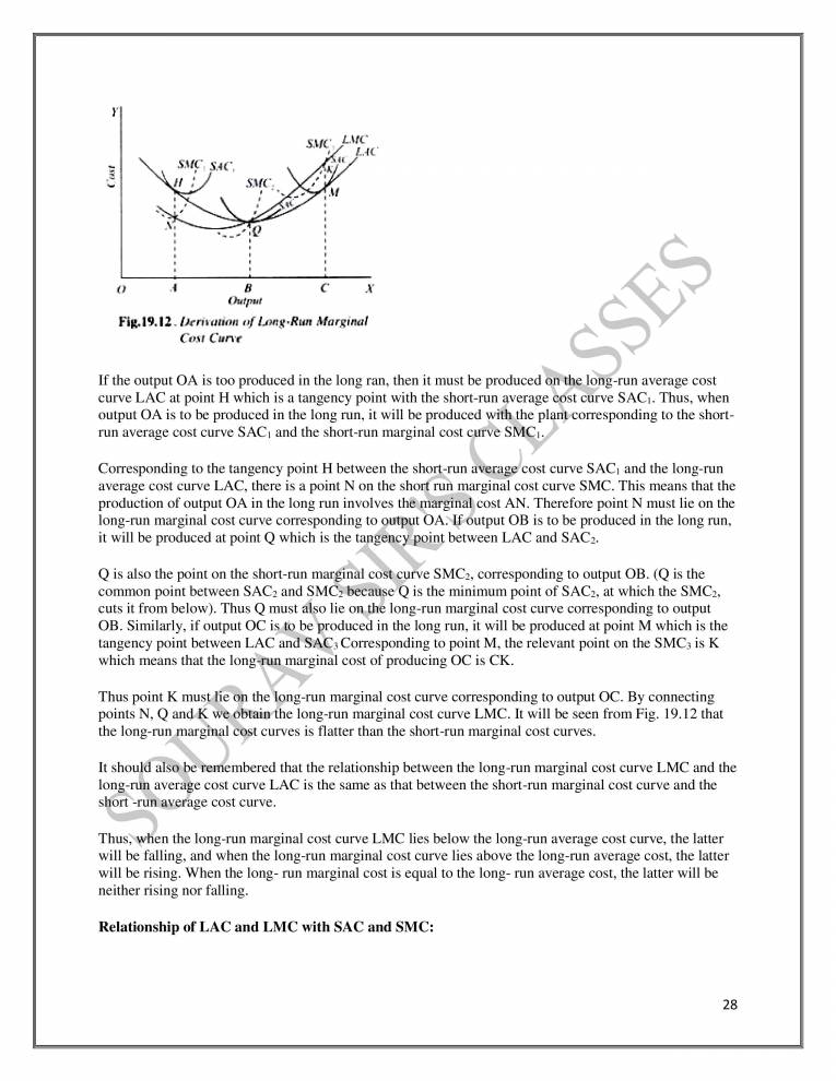
  28. S.WC, SAC, o SMC Output L.wC SVC LAC c Fig. 19.12 Dern-turon of Long-Rem Marginal Cost Curve If the output OA is too produced in the long ran, then it must be produced on the long-run average cost curve LAC at point H which is a tangency point with the short-run cost curve SACI. Thus, when output OA is to be produced in the long run, it will be produced with the plant corresponding to the short- run average cost curve SACI and the short-run marginal cost curv SMCI. Corresponding to the tangency point H between the short-run averag cost curve SACI and the long-run average cost curve LAC, there is a point N on the sho ru marginal cost curve SMC. This means that the production of output OA in the long run involves the g!larginal cost AN. Therefore point N must lie on the long-run marginal cost curve corresponding to output OA:If utput 0B is to be produced in the long run, it will be produced at point Q which is the tangency pp!y! between LAC and SAC2. Q is also the point on the short-run margmal cost curve SMC2, corresponding to output OB. (Q is the common point between SAC2 and SMC2 because Q is the minimum point of SAC2, at which the SMC2, cuts it from below). Thus Q must also lie on the long-run marginal cost curve corresponding to output OB. Similarly, if output OC is to be roduced in the long run, it will be produced at point M which is the tangency point between LAC and SAC3 Corresponding to point M, the relevant point on the SMC3 is K which means that the long-run marginal cost of producing OC is CK. Thus point K must lie on the ong-run marginal cost curve corresponding to output OC. By connecting points N, Q andK we Obtain the long-run marginal cost curve LMC. It will be seen from Fig. 19.12 that the long-run margmal cost curves is flatter than the short-run marginal cost curves. It shoul also be remembered that the relationship between the long-run marginal cost curve LMC and the long-run avera;e cost curve LAC is the same as that between the short-run marginal cost curve and the short -run average cost curve. Thusöwhen the long-run marginal cost curve LMC lies below the long-run average cost curve, the latter will be falling, and when the long-run marginal cost curve lies above the long-run average cost, the latter will be rising. When the long- run marginal cost is equal to the long- run average cost, the latter will be neither rising nor falling. Relationship of LAC and LMC with SAC and SMC: 28
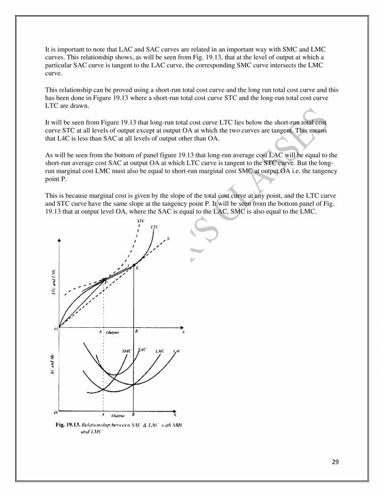
  29. It is important to note that LAC and SAC curves are related in an important way with SMC and LMC curves. This relationship shows, as will be seen from Fig. 19.13, that at the level of output at which a particular SAC curve is tangent to the LAC curve, the corresponding SMC curve intersects the LMC curve. This relationship can be proved using a short-run total cost curve and the long run total cost curve and this has been done in Figure 19.13 where a short-run total cost curve STC and the long-run total cost curve LTC are drawn. It will be seen from Figure 19.13 that long-run total cost curve LTC lies below the short- n tota coy curve STC at all levels of output except at output OA at which the two curves are tangen This means that L4C is less than SAC at all levels of output other than OA. As will be seen from the bottom of panel figure 19.13 that long-run average cos AC yyi!! e equal to the short-run average cost SAC at output OA at which LTC curve is tangent to the STC curve. But the long- run marginal cost LMC must also be equal to short-run marginal cost SM at outputOA i.e. the tangency point P. This is because marginal cost is given by the slope of the total cosVcurve at any point, and the LTC curve and STC curve have the same slope at the tangency point P. It will be seen from the bottom panel of Fig. 19.13 that at output level OA, where the SAC is equal to the LAC, sue is also equal to the LMC. Sit s.wc o 19.13, SMC 29
  30. Economies of Scope WRITE A COMMENT Economies of scope are cost advantages that result when firms provide a variety of products rather than specializing in the production or delivery of a single product or service. Economies of scope also exist if a firm can produce a given level of output of each product line more cheaply than a combination of separate firms, each producing a single product at the given output level. Economies of scope can arise from the sharing or joint utilization of inputs and lead to reductions in unit costs. Scope economies are requently documented in the business literature and have been found to exist in countries, electroni%based B2B (business-to-business) providers, home healthcare, banking, publishing, distribution, and telecommunications. METHODS OF ACHIEVING ECONOMIES OF SCOPE Flexible Manufacturing The use of flexible processes and flexible manufacturing systemyhas resulte in economies of scope because these systems allow quick, low-cost switching of one product lintßo another. If a producer can manufacture multiple products with the same equipment and if the eq ipment allows the flexibility to change as market demands change, the manufacturer can add a variet of new products to their current line. The scope of products increases, offering a barrie to ntry for new firms and a competitive synergy for the firm itself. Related Diversification Economies of scope often result from a related diversification strategy and may even be termed "economies of diversification. " This strategy is made operational when a firm builds upon or extends existing capabilities, resources, o areas of expertise for greater competitiveness. According to Hill, Ireland, and Hoskisson in their best selling strategic management textbook, Strategic Management: Competitiveness and Globalization, firms select related diversification as their corporate-level strategy in an attempt to exploit economies of scope between their various business units. Cost-savings result when a business transfers expertise one business to a new business. The businesses can share operational skills and know-how irvnanufacturing or even share plant facilities, equipment, or other existing assets. They may also share intangible assets like expertise or a corporate core competence. Such sharing of activities is common and is ay to maximize limited constraints. As an example, Kleenex Corporation manufactures a number of paper products for a variety of end users, including products targeted specifically for hospitals and health care providers, infants, children, families, and women€Tfieir brands include Kleenex, Viva, Scott, and Cottonelle napkins, paper towels, and facial tissues; Depends and Poise incontinence products; Huggies diapers and wipes; Pull-Ups, Goodnites, and Little >wlmmers infant products; Kotex, New Freedom, Litedays, and Security feminine hygiene products; and a number of products for surgical use, infection control, and patient care. All of these product lines utilize similar raw material inputs and/or manufacturing processes as well as distribution and logistics channels. 30
  31. Mergers The merger wave that swept the United States in the late 1990s and early 2000s is, in part, an attempt to create scope economies. Mergers may be undertaken for any number of reasons. "As a rule of thumb," explained Rob Preston in an article about the trouble with mergers, scope' acquisitions—moves that enhance or extend a vendor's product portfolio succeed more often than those undertaken to increase size and consolidate costs. " Pharmaceutical companies, for example, frequently combine forces to share research and development expenses and bring new products to market. Research has shown that firms involved in drug discovery realize economies of scope by sustaining diverse portfolios of researc projects that capture both internal and external knowledge spillovers. Linked Supply Chains Today's linked supply chains among raw material suppliers, other vendors, manufacturers holesalers, distributors, retailers, and consumers often bring about economies of scope. Integrating a vertical supply chain results in productivity gains, waste reduction, and cost improvement These •mprovements, which arise from the ability to eliminate costs by operating two or more businesse under the same corporate umbrella, exist whenever it is less costly for two or more businesses to ope a e under centralized management than to function independently. The opportunity to gain cost savings can arise from interrelationships anywhere along a value chain. As firms become linked in supply chains, particularly as par f the new information economy, there is a growing potential for economies of scope. Scope economies can increase a firm's value and lead to increases in performance and higher returns to shareholders.uilding economies of scope can also help a firm to reduce the risks inherent in producing a single product or providing a service to a single industry. 31